An Overview of Cubist
Cubist is a tool for generating rule-based predictive models from data. Whereas its sister system See5/C5.0 produces classification models that predict categories, Cubist models predict numeric values. This short tutorial introduces Cubist's capabilities and explains how to use the system effectively.
In this tutorial, file names and Cubist input appear in
blue fixed-width font
while file extensions and other general forms
are shown highlighted in green.
Buttons and options on the Windows GUI are in maroon.
- Preparing Data for Cubist
- User Interface
- Constructing Models
- Cross-Referencing Models and Data
- Generating Models in Batch Mode
- Linking to Other Programs
Preparing Data for Cubist
We will illustrate Cubist using a simple application -- modeling automobiles' annual fuel cost using data published in 2008 by the US Department of Energy and the US Environmental Protection Agency. Each data point concerns one automobile and the attributes or properties capture (possibly) relevant information as follows:
	Attribute                      Case 1     Case 2     Case 3   .....

	class                          SUV        VAN        CAR
	model                          HUMMER H3  GMC G1500  DODGE CHARGER
	displacement (l)               3.7        5.3        3.5
	cylinders                      4          8          6
	drive                          Auto       Auto       Auto
	gears                          4          4          5
	transmission                   4WD        RWD        4WD
	fuel                           regular    regular    regular
	charger (super- or turbo-)     none       none       none
	valves/cylinder                2          2          4
	displacement/cylinder          0.93       0.66       0.58

	annual fuel cost               2801       3900       2335
Each case has a target attribute or dependent variable -- here the estimated annual fuel cost to run the automobile -- and the other attributes provide information that may help to predict this value, although some automobiles may have unknown values for some attributes. There are only twelve attributes in this example including the target attribute, but Cubist can deal with thousands of attributes if necessary.
Cubist's job is to find how to estimate a case's target value in terms of its attribute values -- here, to relate annual fuel cost to the other information provided for the automobile. Cubist does this by building a model containing one or more rules, where each rule is a conjunction of conditions associated with a linear expression. The meaning of a rule is that, if a case satisfies all the conditions, then the linear expression is appropriate for predicting the target value. A Cubist model thus resembles a piecewise linear model, except that the rules can overlap. As we will see, Cubist can also construct multiple models and can combine rule-based models with instance-based (nearest neighbor) models.
Application files
Every Cubist application has a short name called a filestem; we will use the filestemfc2008
for this illustration.
All files read or written by Cubist for an application
look like filestem.extension,
where filestem identifies the application and
extension describes the contents of the file.
Here is a summary table of the extensions used by Cubist (to be described in later sections):
| names | description of the application's attributes | [required] |
| data | cases used to generate a model | [required] |
| test | unseen cases used to test a model | [optional] |
| cases | cases to be modeled subsequently | [optional] |
| model | rule-based model produced by Cubist | [output] |
| pred | actual and predicted target values for any test cases | [output] |
| out | report produced when a model is generated | [output] |
| set | settings used for the last model | [output] |
APP.DATA,
app.data, and App.Data, are all different.
It is important that the extensions are written in lower case
exactly as shown above, otherwise Cubist will not recognize
the files for your application.
If Cubist cannot seem to find your files even though the filestem
and extensions are correct, please
check that file extensions are not hidden on your computer.
(If extensions are hidden and you write a text file from Wordpad,
it automatically adds an extension .txt that makes the file
invisible to Cubist.)
First, uncheck the "Hide extensions for known file types" box in the
"View" tab of the folder options for your version of Windows.
Then remove any unwanted .txt from your Cubist file names.
All files for an application must be kept together in one folder but several applications can share the same folder.
Names file
The first essential file is
the names file (e.g. fc2008.names) that
defines the attributes used to describe each case.
There are two important subgroups of attributes:
- The value of an explicitly-defined attribute is given directly in the data. A discrete attribute has a value drawn from a set of nominal values, a continuous attribute has a numeric value, a date attribute holds a calendar date, a time attribute holds a clock time, a timestamp attribute holds a date and time, and a label attribute serves only to identify a particular case.
- The value of an implicitly-defined attribute is specified by a formula. (Most attributes are explicitly defined, so you may never need implicitly-defined attributes.)
The file fc2008.names looks like this:
| Data extracted from the site http://www.fueleconomy.gov provided by
| the US Department of Energy and the US Environmental Protection Agency.

fuel cost.                                | target

class:          CAR, STATION WAGON, SUV,
                PICKUP TRUCK, VAN.
model:          label.
displ:          continuous.               | engine displacement (liters/litres)
cylinders:      continuous.
drive:          Auto, Manual.
gears:          continuous.               | 'N/A' if no conventional gears
transmission:   F, R, 4.                  | front, rear, 4WD
fuel:           R, P, D, E, C.            | regular, premium, diesel, ethanol, lpg
charger:        T, S, -.                  | turbo, super, none
fuel cost:      continuous.               | estimated annual fuel cost ($)
valves/cyl:     continuous.               | valves per cylinder

displ/cyl := displ / cylinders.           | displacement per cylinder
Some of the attribute names have been abbreviated and the target
attribute fuel cost appears among the others rather
than at the end.
What's in a name?
Names, labels, and discrete values are represented by arbitrary strings of characters, with some fine print:- Tabs and spaces are permitted inside a name or value, but Cubist collapses every sequence of these characters to a single space.
- Special characters (comma, colon, period, vertical bar `
|') can appear in names and values, but must be prefixed by the escape character `\'. For example, the name "Filch, Grabbit, and Co." would be written as` . (However, it is not necessary to escape colons in times and periods in numbers.)Filch\, Grabbit\, and Co\.'
|'
causes the remainder of the line to be ignored and is handy for
including comments.
When used in this way, `|' should not occur inside a value.
The first important entry of the names file identifies the
attribute that
contains the target value -- the value to be modeled in terms of the
other attributes -- here, fuel cost.
This attribute must be of type continuous or an
implicitly-defined attribute that has numeric values (see below).
Following this entry, all attributes are defined in the order that their values will be given for each case.
Explicitly-defined attributes
The name of each explicitly-defined attribute is followed by a colon `:' and a description of the values taken by the attribute. The attribute name is arbitrary, except that each attribute must have a distinct name, and the namecase weight
is reserved for setting weights for individual cases.
There are eight possibilities:
continuous- The attribute takes numeric values.
date- The attribute's values are dates in the form YYYY/MM/DD
or YYYY-MM-DD,
e.g.
1999/09/30or1999-09-30. Valid dates range from the year 1601 to the year 4000. time- The attribute's values are times in the form HH:MM:SS
with values between
00:00:00and23:59:59. timestamp- The attribute's values are times in the form
YYYY/MM/DD HH:MM:SS or
YYYY-MM-DD HH:MM:SS,
e.g.
1999-09-30 15:04:00. (Note that there is a space separating the date and time.) - a comma-separated list of names
- The attribute takes discrete values, and these are the allowable values.
The values may be prefaced by
[ordered]to indicate that they are listed in a meaningful order, otherwise they will be taken as unordered. For instance, the valueslow, medium, highare ordered, whilemeat, poultry, fish, vegetablesare not. If the attribute values have a natural order, it is better to declare them as ordered so that this information can be exploited by Cubist. discreteN for some integer N- The attribute also takes discrete values, but the values are assembled from the data itself; N is the maximum number of such values. (This is not recommended, since the data cannot be checked, but it can be handy for discrete attributes with many values.)
ignore- The values of the attribute should be ignored.
label- This attribute contains an identifying label for each case, such as an account number or an order code. The value of the attribute is ignored when models are constructed, but is used when referring to individual cases. A label attribute can make it easier to locate errors in the data and also helps with cross-referencing of results to individual cases. If there are two or more label attributes, only the last is used.
Attributes defined by formulas
The name of each implicitly-defined attribute is followed by `:=' and then a formula defining the attribute value. The formula is written in the usual way, using parentheses where needed, and may refer to any attribute that has been defined before this one. Constants in the formula can be `?' (meaning unknown),
`N/A' (meaning not applicable),
numbers (written in decimal notation), dates, times,
and discrete attribute values
enclosed in string quotes `"'.
The operators and functions available for use in the formula are
-
+,-,*,/,%(mod),^(meaning `raised to the power') -
>,>=,<,<=,=,<>or!=(the last two both meaning `not equal') -
and,or -
sin(...),cos(...),tan(...),log(...),exp(...),int(...)(meaning `integer part of')
displ/cyl).
This is a numeric attribute since its value is a ratio of
two explicitly-defined numeric attributes.
The value of a hypothetical attribute
small := cylinders = 4 and class = "CAR".
t or f
since the value given by the formula is either true or false.
If the value of the formula cannot be determined for a particular
case, the value of the implicitly-defined attribute is unknown.
For example, consider a car with a value `?'
for the cylinders attribute.
The displacement per cylinder cannot then be calculated,
so the implicitly-defined attribute displ/cyl would
also have an unknown value.
Dates, times, and timestamps
Dates are stored by Cubist as the number of days since a particular starting point so some operations on dates make sense. Thus, if we have attributes
	d1: date.
	d2: date.
	interval := d2 - d1.
	gap := d1 <= d2 - 7.
	d1-day-of-week := (d1 + 1) % 7 + 1.
interval then represents the number of days from
d1 to d2 (non-inclusive) and
gap would have a true/false value signaling whether
d1 is at least a week before d2.
The last definition is a slightly non-obvious way of determining
the day of the week on which d1 falls, with values
ranging from 1 (Monday) to 7 (Sunday).
Similarly, times are stored as the number of seconds since midnight.
If the names file includes
	start: time.
	finish: time.
	elapsed := finish - start.
elapsed is the number of seconds
from start to finish.
Timestamps are a little more complex. A timestamp is rounded to
the nearest minute, but limitations on the precision of floating-point
numbers mean that the values stored for timestamps from more than
thirty years ago are approximate.
If the names file includes
	departure: timestamp.
	arrival: timestamp.
	flight time := arrival - departure.
flight time is the number of minutes
from departure to arrival.
Selecting the attributes that can appear in models
An optional final entry in the names file affects the way that Cubist constructs models. This entry takes one of the forms
	attributes included:
	attributes excluded:
Excluding an attribute from models is not the same as ignoring the
attribute (see `ignore' above).
As an example, suppose that a numeric attribute A
is defined in the data, but background knowledge suggests that
only the logarithm of A should appear in models.
The names file might then contain the following entries:
	   . . .
	A: continuous.
	LogA := log(A).
	   . . .
	attributes excluded: A.
A could not be defined
as ignore because the definition of LogA
would then be invalid.
The same pattern could be used if the goal was to model the log of
A rather than the value of A itself.
In this case the target attribute would be given as LogA
and the exclusion of A would be necessary to prevent
the value of A being used in the model for LogA.
Data file
The second essential file, the application's data file (herefc2008.data),
provides information on the
training
cases that Cubist will use to construct a model.
The entry for each case consists of one or more lines that give
the values for all explicitly-defined attributes.
Values are separated by commas and the entry for each case
is optionally terminated by a period.
Once again, anything on a line after a vertical bar is ignored.
(If the information for a case occupies more than one line, make sure
that the line breaks occur after commas.)
The first three cases from file fc2008.data are:
SUV,HUMMER H3 4WD,3.7,5,Auto,4,4,R,-,2801,2
VAN,GMC G1500/2500 SAVANA 2WD PASS,5.3,8,Auto,4,R,E,-,3900,2
CAR,DODGE CHARGER AWD,3.5,6,Auto,5,4,R,-,2335,4
Notice that the value of the implicitly-defined attribute
displ/cyl
is not given for each case since it is computed from other attribute values.
Don't forget the commas between values! If you leave them out, Cubist will not be able to process your data.
A value that is missing or unknown is entered as `?'.
Similarly, `N/A' denotes a value that is not applicable for
a particular case.
Test and cases files (optional)
Of course, the value of predictive models lies in their ability to make accurate predictions! It is difficult to judge the accuracy of a model by measuring how well it does on the cases used in its construction; the performance of the model on new cases is much more informative.
The third kind of file used
by Cubist is a test file
of new cases (here fc2008.test) on which the model
can be evaluated.
This file is optional and has
exactly the same format as the data file.
In this application the 1,141 cases have been split randomly 70%:30% into
data and test files containing 800
and 341 cases respectively.
Another optional file, the cases file
(e.g. fc2008.cases),
has the same format as the data and test files.
The cases file is used primarily with
the cross-referencing procedure and public source code,
both of which are
described later on.
User Interface
It is difficult to see what is going on in an interface without
actually using it. As a simple illustration, here is the main window
of Cubist after the fc2008 application has been selected:
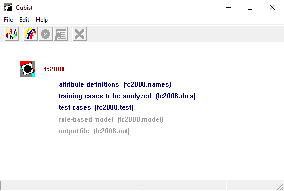
The main window of Cubist has five buttons on its toolbar. From left to right, they are
- Locate Data
- invokes a browse dialog to find the files for your application, or to change the current application;
- Build Model
- selects the type of model to be constructed and sets other options;
- Stop
- interrupts the model-generating process;
- Review Output
- re-displays the output from the last model construction (if any);
- Cross-Reference
- maps between data and models.
The Edit menu facilitates changes to the names file after an application has been located. On-line help is available through the Help menu.
Constructing Models
Once the names, data, and optional files have been set up, everything is ready to use Cubist.
The first step is to locate the date using the Locate Data
button on the toolbar (or the corresponding selection from
the File menu).
We will assume that the fc2008.data file above has been
located in this manner.
There are several options that affect the type of model that Cubist produces and the way that it is constructed. The Construct Model button on the toolbar (or selection from the File menu) displays a dialog box that sets out these model construction options:
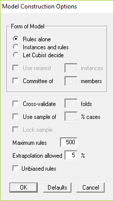
In this section we will examine each of them, starting with the simpler situations.
Rule-based models
When Cubist is invoked with the default values of all options, it constructs a rule-based model and produces output like this:
Cubist [Release 2.10] Tue Jun 11 20:59:46 2019
Target attribute `fuel cost'
Replacing unknown attribute values:
`valves/cyl' by 3.466667
Read 800 cases (12 attributes) from fc2008.data
Model:
Rule 1: [142 cases, mean 1896.5, range 884 to 2801, est err 127.3]
if
class in {CAR, VAN}
displ <= 4.6
fuel in {R, D, C}
then
fuel cost = -50.1 + 162 cylinders + 1293 displ/cyl + 80 displ
+ 47 valves/cyl
Rule 2: [138 cases, mean 2971.4, range 2335 to 4090, est err 227.3]
if
displ > 4.6
displ <= 6.2
gears <= 6
fuel in {R, P}
then
fuel cost = 1010.3 + 284 displ + 91 cylinders - 791 displ/cyl
+ 56 valves/cyl
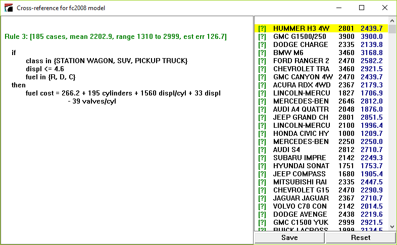
Rule 3: [185 cases, mean 2202.9, range 1310 to 2999, est err 126.7]
if
class in {STATION WAGON, SUV, PICKUP TRUCK}
displ <= 4.6
fuel in {R, D, C}
then
fuel cost = 266.2 + 195 cylinders + 1560 displ/cyl + 33 displ
- 39 valves/cyl
Rule 4: [65 cases, mean 1996, range 1404 to 2502, est err 122]
if
cylinders <= 4
fuel in {P, E}
then
fuel cost = 28532.5 + 10271 displ - 6839 cylinders - 39685 displ/cyl
Rule 5: [13 cases, mean 3900, range 3900 to 3900, est err 0]
if
class in {SUV, PICKUP TRUCK}
displ <= 5
fuel = E
then
fuel cost = 3900
Rule 6: [16 cases, mean 3414.6, range 2999 to 3900, est err 60]
if
class in {SUV, PICKUP TRUCK}
displ > 5
fuel = E
then
fuel cost = -6038.9 + 29563 displ/cyl - 1929 displ
Rule 7: [176 cases, mean 2357.1, range 1876 to 3460, est err 148.4]
if
class in {CAR, STATION WAGON}
displ <= 4.6
cylinders > 4
fuel in {P, E}
then
fuel cost = -309.5 + 376 cylinders - 281 displ + 2293 displ/cyl
Rule 8: [11 cases, mean 3803.2, range 3545 to 3900, est err 116.2]
if
class = VAN
displ > 4.6
fuel = E
then
fuel cost = 3652.1 + 25 cylinders + 20 displ - 88 displ/cyl
Rule 9: [10 cases, mean 3628.9, range 2502 to 4500, est err 467.3]
if
displ > 6.2
then
fuel cost = 7497.8 - 502 displ - 400 displ/cyl + 18 valves/cyl
Rule 10: [15 cases, mean 3024.2, range 2646 to 3460, est err 203.8]
if
displ > 4.6
gears > 6
then
fuel cost = 2144.6 + 1293 displ - 7403 displ/cyl - 334 valves/cyl
Rule 11: [26 cases, mean 2661.6, range 1800 to 3213, est err 233.6]
if
class in {SUV, VAN}
displ <= 4.6
cylinders > 4
fuel in {P, E}
then
fuel cost = 1025 + 362 displ + 59 cylinders
Rule 12: [3 cases, mean 2032.7, range 1999 to 2100, est err 67.3]
if
displ > 4.6
gears = N/A
then
fuel cost = 1969 + 5 displ
Evaluation on training data (800 cases):
Average |error| 142.6
Relative |error| 0.31
Correlation coefficient 0.94
Attribute usage:
Conds Model
96% fuel
92% 98% displ
71% class
33% 98% cylinders
20% gears
95% displ/cyl
61% valves/cyl
Evaluation on test data (341 cases):
Average |error| 152.6
Relative |error| 0.35
Correlation coefficient 0.92
Time: 0.0 secs
The first part identifies the version of Cubist, the run date,
and the attribute that contains the target value.
Now we come to the training data.
Some attribute values might be missing; if so, Cubist replaces
them by the most probable values. Missing values
of continuous attributes are replaced by the mean of
the known values for that attribute, while the replacement for
missing discrete values is the most frequent attribute value.
Any such replacements are noted on the output.
Here valves/cyl is the only explicitly-defined attribute
whose value is missing for some cases in fc2008.data;
those cases are given the average value (a rather unrealistic 3.46667).
The same values are also used to replace missing values in any test cases,
although the messages are not repeated.
Cubist constructs a model from the 800 training cases
in the file fc2008.data, and this appears next.
A model consists of a list of rules, each
of the form
if conditions then linear formula
A rule indicates that, whenever a case satisfies all the conditions,
the linear formula is appropriate for predicting the value of
the target attribute. (If two or more rules apply to
a case, then the values are averaged to arrive at a final
prediction.)
Although the order of the rules does not affect the value predicted by a model, Cubist presents them in decreasing order of importance. The first rule makes the greatest contribution to the model's accuracy on the training data; the last rule has the least impact.
Each rule also carries some descriptive information: the number of training cases that satisfy the rule's conditions, their target values' mean and range, and a rough estimate of the expected error magnitude of predictions made by the rule. Within the linear formula, the attributes are ordered in decreasing relevance to the result.
Let's illustrate all this on Rule 1 above. There are three conditions:
        class in {CAR, VAN}
        displ <= 4.6
        fuel in {R, D, C}
Among the 800 training cases there are 142 that satisfy all three
conditions; their fuel costs range from $884 to $2801 with
an average value of $1896.5. Cubist finds that the target value of
these or other cases satisfying the conditions can be modeled
by the formula
fuel cost = -50.1 + 162 cylinders + 1293 displ/cyl + 80 displ + 47 valves/cyl
with an estimated error of $127.3.
For cases covered by this rule,
cylinders has the most effect on fuel cost,
displ/cyl and displ a lesser effect, and
valves/cyl the least effect.
There is a point worth noting about Rule 5:
  Rule 5: [13 cases, mean 3900, range 3900 to 3900, est err 0.0]

    if
        class in {SUV, PICKUP TRUCK}
        displ <= 5
        fuel = E
    then
        fuel cost = 3900
The formula predicts a constant value for these cases. In rules like
this, the constant value may differ from the mean, which may appear
odd! This is not an error -- under the default option settings, Cubist
attempts to minimize average error magnitude, and so uses the median
target value of the cases covered by the rule
rather than the mean. This can be altered by invoking the option
for unbiased rules, described later.
The next section covers the evaluation of this model shown in the second part of the output. Before we leave this output, though, the final line states the elapsed time for the run. For small applications such as this, with only a few training cases and a handful of attributes, a model is produced quite quickly. Model construction can take much longer for larger applications with many thousands of cases and tens or hundreds of attributes.
Evaluation
Models constructed by Cubist are evaluated on the training data from which
they were generated, and also on a separate file of unseen test cases
if this is present. (Evaluation by cross-validation is discussed
later.)
Results on the cases in fc2008.data are:
Evaluation on training data (800 cases):

    Average  |error|              142.6
    Relative |error|               0.31
    Correlation coefficient        0.94
The average error magnitude is straightforward enough.
The relative error magnitude is the ratio of the average
error magnitude to the error magnitude that would result from
always predicting the mean value;
for useful models, this should be less than 1!
The correlation coefficient measures the agreement between
the cases' actual values of the target attribute and those
values predicted by the model.
Usually, as in this example, the results cover all training cases. When there are more than 20,000 of them and composite models (see later) are used, the evaluation covers only a random sample of 10,000 training cases and this fact is noted in the output.
For some applications, particularly those with many attributes, it may be useful to know how individual attributes contribute to the model. This is shown in the next section:
        Attribute usage:
          Conds  Model

           96%           fuel
           92%    98%    displ
           71%           class
           33%    98%    cylinders
           20%           gears
                  95%    displ/cyl
                  61%    valves/cyl
The first column shows the approximate percentage of cases for which
the named attribute appears in a condition of an applicable rule,
while
the second column gives the percentage of cases for which the attribute
appears in the linear formula of an applicable rule. The
second entry, for example, says that displ is used in
the condition part of rules that cover 92% of cases and in the formulas
of rules that cover 98% of cases.
Attributes for which both these values are less than 1% are not shown.
If a test file is present, Cubist produces a summary similar to that for the training cases:
Evaluation on test data (341 cases):

    Average  |error|              152.6
    Relative |error|               0.35
    Correlation coefficient        0.92
Cubist also generates a file
filestem.pred (here fc2008.pred)
that shows the actual and predicted value for each test case.
The first few lines of this file generated from the run above are:
(Default value 2419.5)

      Actual     Predicted    Case
       Value         Value
 -----------  ------------    ----
        1751        1736.2    JEEP PATRIOT 2WD
        1680        1592.4    SUZUKI SX4 SEDAN
        1357        1511.8    TOYOTA COROLLA
        2367        2323.3    PORSCHE CARRERA 4 S TARGA
Notice that each case is identified by its value of the
label attribute; if there is no such attribute, the
case number in the .test file is used instead.
Another way of assessing the accuracy of the predictions is
through a visual inspection of a scatter plot
that graphs the real target values of new cases
against the values predicted by the model. When a file
filestem.test of test cases is present,
Cubist also provides
a scatter plot window. In this example, it looks like this:
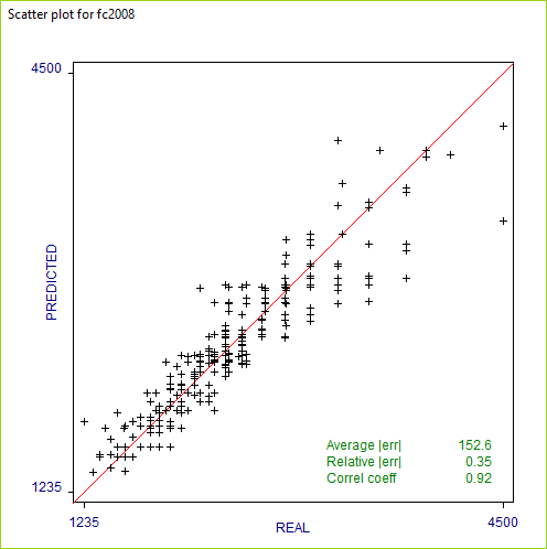
When the number of test cases is very large, the plot shows only a sample of the points.
Unbiased rules
In its default mode, Cubist tries to minimize the average absolute error of the values predicted for new cases. As a consequence, the rules that Cubist generates may be biased -- the mean predicted value for the training cases covered by a rule may differ from their mean value.Suppose, for instance, that we have to summarize the values 1, 2, and 12 by a single number. If we choose the mean value 5, the average absolute error over these values would be 14/3. Choosing the median value 2, however, the average absolute error becomes 11/3. Even though it gives lower absolute error, the choice of 2 is biased since the prediction (2) is lower than the mean of the values (5).
The model construction dialog box contains an option that instructs Cubist to make each rule approximately unbiased, with the downside that average absolute error is usually slightly higher. This option is recommended for applications where the training cases have a preponderance of a single target value (such as zero) because unbiased rules tend to give a finer gradation of predicted values.
When the fuel cost application is run with the option for unbiased rules, the only effect is to change the constant in the formula for each rule and the rule's estimated error. The rule that shows the greatest difference is
  Rule 8: [11 cases, mean 3803.2, range 3545 to 3900, est err 169]

    if
        class = VAN
        displ > 4.6
        fuel = E
    then
        fuel cost = 3555.3 + 25 cylinders + 20 displ - 88 displ/cyl
The constant term in the formula changes from 3652.1 to 3555.3 and the
estimated error is greater. This shows that the original rule was
strongly biased towards higher values. For this application,
unbiased rules have a slightly greater error of 153.1 on the unseen
test cases.
Finally, because cases can be covered by different numbers of rules, the use of unbiased rules does not guarantee that the entire model is unbiased.
Composite models
For some applications, the predictive accuracy of a rule-based model can be improved by combining it with an instance-based or nearest-neighbor model. The latter predicts the target value of a new case by finding the n most similar cases in the training data, and using the (perhaps weighted) average of their target values as the predicted value for the new case.Cubist employs an unusual method for combining rule-based and instance-based models. To predict a value for case C, Cubist first finds the n training cases that are "nearest" (most similar) to C. Cubist then uses the known values of the neighbors, their values as predicted by the model, and the value predicted by the model for C to arrive at a composite prediction.
The model construction dialog box contains three options: to use purely rule-based models, to use composite models as above, or to leave the decision to Cubist itself. In the latter case, Cubist derives from the training data a heuristic estimate of the accuracy of each type of model, and chooses the form that appears more accurate. The derivation of these estimates requires quite a lot of computation, so leaving the decision to Cubist can result in a noticeable increase in the time required to build a model.
Now for the value of n, the number of nearest neighbors to be used. Following the options for model form in the options dialog box above is a (grayed-out) section covering nearest neighbors. If composite models are selected or Cubist is allowed to decide whether to use them, this option becomes active and, when selected, allows the number of nearest neighbors to be entered directly; the allowable range is from 1 to 9. If the value is not specified in this way, Cubist will choose an appropriate value in the range.
To continue the illustration: when Cubist is allowed to choose a model type on the basis of the 800 training cases and the number of nearest neighbors is not specified, it opts for a composite model using a single nearest neighbor. The rule-based model itself is unchanged, but the composite model gives different results on the training and test cases, the latter being
Evaluation on test data (341 cases):

    Average  |error|               99.8
    Relative |error|               0.23
    Correlation coefficient        0.95
The performance of the composite model on the test cases
in fc2008.test thus improves
upon that of the default rule-based model,
average error magnitude falling from 152.6 to 99.8.
Nearest neighbor models are adversely affected by the presence of irrelevant attributes. All attributes are taken into account when evaluating the similarity of two cases and irrelevant attributes introduce a random factor into this measurement. As a result, composite models tend to be more effective when the number of attributes is relatively small and all attributes are relevant to the prediction task.
Committee models
In addition to the composite rule-based/nearest neighbor models discussed above, Cubist can also generate committee models made up of several rule-based models. Each member of the committee predicts the target value for a case and the members' predictions are averaged to give a final prediction.The first member of a committee model is always exactly the same as the model generated without the committee option. The second member is a rule-based model designed to correct the predictions of the first member; if the first member's prediction is too low for a case, the second member will attempt to compensate by predicting a higher value. The third member tries to correct the predictions of the second member, and so on. The recommended number of members is five, a value that balances the benefits of the committee approach against the cost of generating extra models.
The dialog box has a checkbox for selecting committee models and a field for specifying the number of committee members. When this option is invoked with the default five members, the results show a smaller improvement than that obtained with composite models:
Evaluation on test data (341 cases):

    Average  |error|              141.3
    Relative |error|               0.32
    Correlation coefficient        0.94
Committee models are of most benefit when the initial model is reasonably accurate, so they are more useful for fine-tuning good models than for overcoming the deficiencies of poor models. Finally, committee models can be used in conjunction with composite models. (In this application, using a 5-member committee model with instances further reduces error on the test cases to 94.8.)
Simplicity-accuracy trade-off
Cubist employs heuristics that try to simplify models without substantially reducing their predictive accuracy. In some applications, however, it might be desirable to generate more concise models -- for instance, when the models must be very easy to understand. Of course, over-simplified models usually have lower predictive accuracy so there is a trade-off between simplicity and utility.
The complexity of a model can be controlled by restricting the
number of rules that it may contain (the default value being 500 rules).
The dialog box includes a field for specifying the
maximum number of rules that may be used in a model.
For the fc2008 application,
setting the maximum number of rules to 5
gives a simpler model:
  Rule 1: [142 cases, mean 1896.5, range 884 to 2801, est err 127.3]

        class in {CAR, VAN}
        displ <= 4.6
        fuel in {R, D, C}
    then
        fuel cost = -50.1 + 162 cylinders + 1293 displ/cyl + 80 displ
                    + 47 valves/cyl

  Rule 2: [166 cases, mean 2998.8, range 1999 to 4500, est err 264.3]

    if
        displ > 4.6
        fuel in {R, P}
    then
        fuel cost = 1822.4 + 320 displ - 1721 displ/cyl + 89 valves/cyl
                    + 39 cylinders

  Rule 3: [40 cases, mean 3679.2, range 2999 to 3900, est err 222]

    if
        displ > 4.6
        fuel = E
    then
        fuel cost = 4218.9 - 7008 displ + 55286 displ/cyl

  Rule 4: [185 cases, mean 2202.9, range 1310 to 2999, est err 126.7]

    if
        class in {STATION WAGON, SUV, PICKUP TRUCK}
        displ <= 4.6
        fuel in {R, D, C}
    then
        fuel cost = 266.2 + 195 cylinders + 1560 displ/cyl + 33 displ
                    - 39 valves/cyl

  Rule 5: [267 cases, mean 2298.8, range 1404 to 3460, est err 171.2]

    if
        displ <= 4.6
        fuel in {P, E}
    then
        fuel cost = -1661.1 + 581 cylinders - 733 displ + 5358 displ/cyl
The downside in this example is that the average error magnitude on
the test cases increases from 152.6 to 167.0.
Extrapolation
The extrapolation parameter controls the extent to which predictions made by Cubist's models can fall outside the range of values seen in the training data. Extrapolation is inherently more risky than interpolation, where predictions must lie between the lowest and highest observed value.The dialog box contains a field for this extrapolation factor in the form of a percentage. Each rule records the highest and lowest target value of the training cases satisfying that rule's conditions. When the target value of a new case is predicted using the rule, the value computed from the linear formula may fall outside this range. The extrapolation parameter limits the degree to which new values can lie above or below the values seen in the training data, expressed as a percentage of the range (the default being 5%).
For example, the lowest target value among the 142 training cases covered by Rule 1 above is 884 and the highest is 2801. The range is therefore 1917 and, under the default extrapolation limit of 5%, the value predicted by this rule for a new case cannot be lower than 788.15 (884 - 95.85) or higher than 2896.85 (2801 + 95.85). Any computed value that lies outside these bounds is changed to the nearer bound. If the linear formula associated with Rule 1 were to predict a value of 600, say, then this would be adjusted to 788.15.
Extrapolation may be constrained even further in two situations. When all the training cases covered by a rule have target values greater than or equal to zero, the rule will never predict a value less than zero. This restriction prevents Cubist from making silly predictions such as negative fuel costs. Similarly, when a rule covers cases whose target values are all less than or equal to zero, the predicted value from the rule will never be positive.
Sampling from large datasets
Even though Cubist is relatively fast, building models from a large number of cases can take an inconveniently long time. Cubist incorporates a facility to extract a random sample from a dataset, construct a model from the sample, and then test the model on a disjoint collection of cases. By using a smaller set of training cases in this way, the process of generating a model is expedited, but at the cost of a possible reduction in the model's predictive performance.The Sample option with x% has two consequences. Firstly, a random sample containing x% of the cases in the application's data file is used to construct the model. Secondly, the model is evaluated on a non-overlapping set of test cases consisting of another (disjoint) sample of the same size as the training set (if x is less than 50%), or all cases that were not used in the training set (if x is greater than or equal to 50%).
As an example, suppose that the application's data file contains 100,000 cases. If a sample of 10% is used, the model will be constructed from a sample of 10,000 cases and tested on a disjoint sample of 10,000 cases. Alternatively, selecting sampling with 60% will cause the model to be constructed from 60,000 cases and tested on the remaining 40,000 cases.
By default, the random sample changes every time that a model is constructed, so that successive runs of Cubist with sampling will usually produce different results. This re-sampling can be avoided by selecting the Lock sample option that uses the current sample for constructing subsequent models. If this option is selected, the sample will change only when another application is loaded, the sample percentage is altered, the option is unselected, or Cubist is restarted.
Cross-validation trials
As we saw earlier, the performance of a model on the training cases from which it was constructed gives a poor estimate of its accuracy on new cases. The true predictive accuracy of the model can be estimated by sampling, as above, or by using a separate test file; either way, the classifier is evaluated on cases that were not used to build it. However, this estimate can be unreliable unless the numbers of cases used to build and evaluate the model are both large. If the cases infc2008.data and
fc2008.test were to be shuffled
and divided into new training and test sets,
Cubist would probably construct a different model whose accuracy
on the test cases might vary considerably.
One way to get a more reliable estimate of predictive accuracy is by f-fold cross-validation. The cases in the data file are divided into f blocks of roughly the same size and target value distribution. For each block in turn, a model is constructed from the cases in the remaining blocks and tested on the cases in the hold-out block. In this way, each case is used just once as a test case. The accuracy of a model produced from all the cases is estimated by averaging results on the hold-out cases.
Running a 10-fold cross-validation using the default options gives results on the hold-out cases similar to these:
Summary:

    Average  |error|              149.4
    Relative |error|               0.33
    Correlation coefficient        0.92
The file fc2008.out contains the results
of all cross-validation folds and the
file fc2008.pred shows a case-by-case
summary of the performance of the Cubist models on unseen cases.
A scatter plot of performance on the unseen cases is also provided.
A different random partition of the training cases is used every time a cross-validation is run. The whole cross-validation can be repeated a few times and results averaged to give a more reliable estimate.
Since a single cross-validation fold uses only part of the application's data, running a cross-validation does not cause a model to be saved. To save a model for later use, simply run Cubist without employing cross-validation.
Weighting individual cases
By default, all training cases are treated equally when a model is constructed. In some applications, however, it may be desirable to assign different importance to the cases. Cubist achieves this by recognizing an optional attribute that gives the weight of each case. The attribute name must becase weight and it must have numeric values.
The relative weight
assigned to each case is its value of this attribute divided by
the average value; if the value is undefined ("?"),
not applicable ("N/A"), or is less than or equal to zero,
the case's relative weight is set to 1.
The case weight attribute itself is not used in the model!
To illustrate the idea, let us suppose that we wish our model
to be relatively more accurate on cars rather than other vehicle types.
We might add a case weight attribute of type continuous
to fc2008.names
and add an extra value to each case in the .data
file, 5 for cars and 1 for other vehicles.
This means that the importance of a training case for a car
is five times that of cases for other vehicle types.
Cubist will now attempt to minimize
weighted error, so cars should have more
influence on the new model.
(Note: we must also add an extra value to each case in the
.test file, since we have increased the number of
attributes. This value is not used.)
The initial model gives an average absolute error of 161.0 for the cars in the unseen test cases. With the case-weighted model, this error drops to 153.1.
A cautionary note: The use of case weighting does not guarantee that the model will be more accurate for unseen cases with higher weights. Predictive accuracy on more important cases is likely to be improved only when cases with similar values of the predictor attributes also have similar values of the case weight attribute, i.e. when relatively important cases "clump together." Without this property, case weighting can introduce an unhelpful element of randomness into the model generation process.
Cross-Referencing Models and Data
Cubist incorporates a helpful facility that links data and the
relevant model rules.
We will illustrate this facility using the first run
with the fc2008 application.
The Cross-Reference button brings up a
dialog asking the user to choose a file from among
filestem.data,
filestem.test, and
filestem.cases.
(This dialog is skipped if only one of these files is present.)
For this example we have used the data file from
which the model was generated.
Cubist then shows a window containing the most recent model for the current application and a list of the selected cases. Each case listing has an identifying label or index number, the case's actual target value, and, in blue, the target value predicted for it by the most recent model.
Clicking on a case number or label shows the rules relevant to that case. Clicking on the first case shows that it is covered by Rule 3:
Click on any rule to show all the cases covered by that rule. For instance, clicking on Rule 12 shows the 3 training cases that satisfy the conditions of that rule:
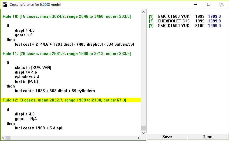
Finally, clicking on the text [?] in front of a case number or label displays that case:
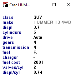
The values of label attributes and any attributes ignored or excluded are displayed in a lighter tone to indicate that they play no part in modeling the case.
The Save button preserves the details of the displayed model and case list as an ASCII file. The Reset button restores the window to its initial state.
Generating Models in Batch Mode
The Cubist distribution includes a program CubistX that
can be used to produce models non-interactively.
This console application resides in the same folder as Cubist
(usually C:\Program Files\Cubist for single-computer licensees
or the Cubist folder on your desktop for network licences)
and is invoked from
an MS-DOS Prompt window. The command to run the program is:
start /B CubistX -f filestem parameters
where the parameters enable one or more options to
be selected:
-u
| generate unbiased rules |
-i
| use instances and rules (composite models) |
-a
| allow the use of instances and rules |
-n neighbors
| set the number of nearest neighbors (1 to 9) |
-C members
| construct a committee model |
-S percent
| use the sampling option |
-I seed
| set the sampling seed value |
-X folds
| carry out a cross-validation |
-r rules
| set the maximum number of rules |
-e percent
| set the extrapolation limit |
If desired, output from Cubist can be diverted to a file in the usual way.
Linking to Other Programs
The most recent model generated by Cubist is saved in file
filestem.model.
Free C source code is available to read these model files and
to make predictions with them, enabling you to
use Cubist models in other programs.
As an example, the source includes a program sample.c that reads a saved model file and then prints the value predicted by the model for each case in a cases file. This sample program is intended to illustrate methods for interacting with the model.
The program expects to find the following files:
-
filestem
.model, the model file generated by Cubist. -
filestem
.names, the names file as it was when the model was generated. -
filestem
.data, the training data (required only if the model is a composite instances-and-rules model). -
filestem
.cases, the cases for which predicted values are required. This file has the same format as a.datafile, except that the value of the target attribute can be unknown (?).
There are several options that control the format of the output:
-f filestem
| identify the application (required) |
-p
| show the saved model |
-e
| show estimated error bounds for each prediction in the form
+-E
|
-i
| for composite models, show each nearest neighbor and its distance from the case |
E
for about 95% of cases. A summary at the end of the output shows the
actual percentage of cases whose true value is known and
lies within the given bounds.
As an example, we use the original model for fc2008 and
copy the .test file into fc2008.cases.
When the -e option is selected, the (abbreviated)
output looks like this:
Case                  Actual    Predicted
 ID                    Value        Value

 JEEP PATRIOT 2         1751       1736.2 +- 316.8
 SUZUKI SX4 SED         1680       1592.4 +- 318.2
 TOYOTA COROLLA         1357       1511.8 +- 318.2
     . . . . .
*BUGATTI VEYRON         4500       3353.8 +- 1168.2
     . . . . .
 HONDA ELEMENT          1911       1905.4 +- 316.8
 FORD F150 STX          2801         2902 +- 568.2

318 / 341 (93%) cases within error bounds
The asterisk in the first column of the Bugatti case indicates that
its value for one or more of the attributes used in the model lies
outside the range observed in the training data, so the predicted
value is suspect. (It has 16 cylinders, whereas none of the training
cases has more than 12.)
Click
here to download a zip archive
containing the C source code.
Please see the comments at the beginning of sample.c
for information on compiling the program.
The archive includes CubistSam.exe, a pre-compiled
version of the sample program. Instructions for running this as
a console application are given in the file CubistSam.txt.
| © RULEQUEST RESEARCH 2019 | Last updated June 2019 |
| home | products | download | evaluations | prices | purchase | contact us |